Exercice 48

1. L'application est symétrique, et linéaire par rapport à $f$, par linéarité de la dérivation et de l'intégrale. Pour $f \in E$, la fonction $f^{2} + f'^{2}$ est continue et positive, donc $\langle f, f \rangle \geqslant 0$. Si $\langle f, f \rangle = 0$, le théorème 4 du chapitre 18 montre que $f^{2} + f'^{2}$ est nulle sur $[0\,,1]$, donc $f = 0$. $$\boxed{\langle f, g \rangle = \int_{0}^{1} (fg + f'g') \text{ est un produit scalaire sur } \mathcal{C}^{1}([0\,,1], \mathbb{R})}$$

2. L'équation $y'' - y = 0$ est linéaire, homogène, à coefficients constants, d'équation caractéristique $r^{2} - 1 = 0$, de racines $\pm 1$ (chapitre 6, théorème 5) : ses solutions sont les fonctions $\lambda\mathrm{e}^{t} + \mu\mathrm{e}^{-t}$, c'est-à-dire les combinaisons linéaires de $\operatorname{ch}$ et $\operatorname{sh}$. Ainsi $F = \mathrm{Vect}(\operatorname{ch}, \operatorname{sh})$ est un sous-espace de $E$, et la famille $(\operatorname{ch}, \operatorname{sh})$ est libre : si $a\operatorname{ch} + b\operatorname{sh} = 0$, l'évaluation en $0$ donne $a = 0$, puis celle en $1$ donne $b = 0$. Donc $\boxed{\dim F = 2}$, ce que donnait aussi la proposition 1 (ii) du chapitre 15.

Soit $f \in E$ et $g \in F$. On intègre par parties $\int_{0}^{1} f'g'$, en primitivant $f'$ et en dérivant $g'$, qui est de classe $\mathcal{C}^{1}$ puisque $g'' = g$ (chapitre 6, proposition 4) : $$\int_{0}^{1} f'g' = \big[fg'\big]_{0}^{1} - \int_{0}^{1} fg'' = f(1)g'(1) - f(0)g'(0) - \int_{0}^{1} fg, \qquad\text{d'où}\qquad \boxed{\langle f, g \rangle = f(1)g'(1) - f(0)g'(0)}$$ Si $f(0) = f(1) = 0$, ce produit est nul pour tout $g \in F$, et $f \in F^{\perp}$. Réciproquement, si $f \in F^{\perp}$, le choix $g = \operatorname{ch}$, avec $g' = \operatorname{sh}$ et $\operatorname{sh} 0 = 0$, donne $f(1)\operatorname{sh} 1 = 0$, donc $f(1) = 0$ ; le choix $g = \operatorname{sh}$, avec $g' = \operatorname{ch}$, donne alors $-f(0) = 0$. $$\boxed{F^{\perp} = \{f \in E \mid f(0) = f(1) = 0\}}$$

3. Par la proposition 10 (ii), $p_{F}(f)$ est l'unique $g \in F$ tel que $f - g \in F^{\perp}$, c'est-à-dire tel que $g(0) = f(0)$ et $g(1) = f(1)$. La fonction $t \mapsto \operatorname{sh}(1 - t) = \operatorname{sh} 1\,\operatorname{ch} t - \operatorname{ch} 1\,\operatorname{sh} t$ appartient à $F$, s'annule en $1$ et vaut $\operatorname{sh} 1$ en $0$ ; la fonction $\operatorname{sh}$ s'annule en $0$ et vaut $\operatorname{sh} 1$ en $1$. On en déduit $$\boxed{p_{F}(f)(t) = \frac{f(0)\,\operatorname{sh}(1 - t) + f(1)\,\operatorname{sh} t}{\operatorname{sh} 1}}$$ La projection orthogonale sur $F$ remplace $f$ par l'unique solution de $y'' = y$ qui a les mêmes valeurs aux deux bords.

4. Soit $g_{\alpha, \beta} = \frac{\alpha\,\operatorname{sh}(1 - t) + \beta\,\operatorname{sh} t}{\operatorname{sh} 1}$, qui appartient à $F \cap E_{\alpha, \beta}$. Pour toute $f \in E_{\alpha, \beta}$, la question 3 donne $p_{F}(f) = g_{\alpha, \beta}$, et le théorème de Pythagore, appliqué à $g_{\alpha, \beta} \in F$ et $f - g_{\alpha, \beta} \in F^{\perp}$, donne $$\int_{0}^{1}\big(f^{2} + f'^{2}\big) = \lVert f \rVert^{2} = \lVert g_{\alpha, \beta} \rVert^{2} + \lVert f - g_{\alpha, \beta} \rVert^{2} \geqslant \lVert g_{\alpha, \beta} \rVert^{2},$$ avec égalité si et seulement si $f = g_{\alpha, \beta}$. La borne inférieure est donc un minimum, atteint en la seule fonction $g_{\alpha, \beta}$. Pour le calculer, on applique la formule de la question 2 avec $f = g = g_{\alpha, \beta}$, après avoir dérivé : $$g_{\alpha, \beta}'(t) = \frac{-\alpha\,\operatorname{ch}(1 - t) + \beta\,\operatorname{ch} t}{\operatorname{sh} 1}, \qquad g_{\alpha, \beta}'(0) = \frac{\beta - \alpha\operatorname{ch} 1}{\operatorname{sh} 1}, \qquad g_{\alpha, \beta}'(1) = \frac{\beta\operatorname{ch} 1 - \alpha}{\operatorname{sh} 1},$$

$$\lVert g_{\alpha, \beta} \rVert^{2} = \beta\,\frac{\beta\operatorname{ch} 1 - \alpha}{\operatorname{sh} 1} - \alpha\,\frac{\beta - \alpha\operatorname{ch} 1}{\operatorname{sh} 1}, \qquad \boxed{\inf_{f \in E_{\alpha, \beta}} \int_{0}^{1}\big(f^{2} + f'^{2}\big) = \frac{(\alpha^{2} + \beta^{2})\operatorname{ch} 1 - 2\alpha\beta}{\operatorname{sh} 1}}$$ atteinte seulement en $g_{\alpha, \beta}$. On a contrôlé cette valeur par un calcul direct de l'intégrale pour quatre couples $(\alpha, \beta)$ ✓.

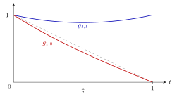
Pour $\alpha = \beta = 1$, en bleu, la fonction optimale est $g_{1, 1}(t) = \frac{\operatorname{ch}(t - 1/2)}{\operatorname{ch}(1/2)}$ : elle descend jusqu'à $\frac{1}{\operatorname{ch}(1/2)} \approx 0{,}887$ au milieu, et le minimum vaut $\frac{2(\operatorname{ch} 1 - 1)}{\operatorname{sh} 1} = 2\,\mathrm{th}\,\frac{1}{2} \approx 0{,}924$, plus petit que la valeur $1$ obtenue pour la fonction constante, en gris. En descendant un peu au milieu, elle gagne plus sur $\int f^{2}$ qu'elle ne perd sur $\int f'^{2}$, qui n'est plus nul mais reste petit. Pour $\alpha = 1$ et $\beta = 0$, en rouge, la fonction optimale $g_{1, 0}(t) = \frac{\operatorname{sh}(1 - t)}{\operatorname{sh} 1}$ est très proche de la droite grise $1 - t$, et les deux valeurs le sont aussi : $\frac{\operatorname{ch} 1}{\operatorname{sh} 1} \approx 1{,}313$ contre $\frac{4}{3} \approx 1{,}333$.

À retenir. L'ensemble $E_{\alpha, \beta} = g_{\alpha, \beta} + F^{\perp}$ est un sous-espace affine de direction $F^{\perp}$ (chapitre 14) ; son élément de plus petite norme est celui qui est orthogonal à la direction. C'est la même idée que la distance à un sous-espace, appliquée à $0$ et à un sous-espace affine. Le produit scalaire de la question 1 n'est pas celui de la proposition 2 : il mesure aussi la dérivée, et c'est pourquoi la fonction optimale est une solution d'équation différentielle, et non une fonction affine.